Pearson’s Contingency Coefficient¶

Module Interface¶

class torchmetrics.PearsonsContingencyCoefficient(num_classes, nan_strategy='replace', nan_replace_value=0.0, **kwargs)[source]

Compute Pearson’s Contingency Coefficient statistic.

This metric measures the association between two categorical (nominal) data series.

$Pearson = \sqrt{\frac{\chi^2 / n}{1 + \chi^2 / n}}$

where

$\chi^2 = \sum_{i,j} \ frac{\left(n_{ij} - \frac{n_{i.} n_{.j}}{n}\right)^2}{\frac{n_{i.} n_{.j}}{n}}$

where $n_{ij}$ denotes the number of times the values $(A_i, B_j)$ are observed with $A_i, B_j$ represent frequencies of values in preds and target, respectively.

Pearson’s Contingency Coefficient is a symmetric coefficient, i.e. $Pearson(preds, target) = Pearson(target, preds)$ .

The output values lies in [0, 1] with 1 meaning the perfect association.

Parameters

num_classes¶ (int) – Integer specifing the number of classes
nan_strategy¶ (Literal[‘replace’, ‘drop’]) – Indication of whether to replace or drop NaN values
nan_replace_value¶ (Union[int, float, None]) – Value to replace NaN``s when ``nan_strategy = 'replace'
kwargs¶ (Any) – Additional keyword arguments, see Advanced metric settings for more info.

Returns

Pearson’s Contingency Coefficient statistic

Raises

ValueError – If nan_strategy is not one of ‘replace’ and ‘drop’
ValueError – If nan_strategy is equal to ‘replace’ and nan_replace_value is not an int or float

Example

>>> from torchmetrics.nominal import PearsonsContingencyCoefficient
>>> _ = torch.manual_seed(42)
>>> preds = torch.randint(0, 4, (100,))
>>> target = torch.round(preds + torch.randn(100)).clamp(0, 4)
>>> pearsons_contingency_coefficient = PearsonsContingencyCoefficient(num_classes=5)
>>> pearsons_contingency_coefficient(preds, target)
tensor(0.6948)

Initializes internal Module state, shared by both nn.Module and ScriptModule.

plot(val=None, ax=None)[source]

Plot a single or multiple values from the metric.

Parameters

val¶ (Union[Tensor, Sequence[Tensor], None]) – Either a single result from calling metric.forward or metric.compute or a list of these results. If no value is provided, will automatically call metric.compute and plot that result.
ax¶ (Optional[Axes]) – An matplotlib axis object. If provided will add plot to that axis

Return type

Tuple[Figure, Union[Axes, ndarray]]

Returns

Figure and Axes object

Raises

ModuleNotFoundError – If matplotlib is not installed

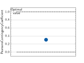
>>> # Example plotting a single value
>>> import torch
>>> from torchmetrics.nominal import PearsonsContingencyCoefficient
>>> metric = PearsonsContingencyCoefficient(num_classes=5)
>>> metric.update(torch.randint(0, 4, (100,)), torch.randint(0, 4, (100,)))
>>> fig_, ax_ = metric.plot()

(Source code, png, hires.png, pdf)

../_images/pearsons_contingency_coefficient-1.png

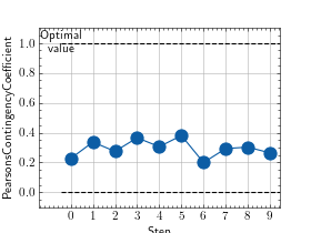
>>> # Example plotting multiple values
>>> import torch
>>> from torchmetrics.nominal import PearsonsContingencyCoefficient
>>> metric = PearsonsContingencyCoefficient(num_classes=5)
>>> values = [ ]
>>> for _ in range(10):
...     values.append(metric(torch.randint(0, 4, (100,)), torch.randint(0, 4, (100,))))
>>> fig_, ax_ = metric.plot(values)

(Source code, png, hires.png, pdf)

../_images/pearsons_contingency_coefficient-2.png

Functional Interface¶

torchmetrics.functional.pearsons_contingency_coefficient(preds, target, nan_strategy='replace', nan_replace_value=0.0)[source]

Compute Pearson’s Contingency Coefficient for measuring the association between two categorical data series.

$Pearson = \sqrt{\frac{\chi^2 / n}{1 + \chi^2 / n}}$

where

$\chi^2 = \sum_{i,j} \ frac{\left(n_{ij} - \frac{n_{i.} n_{.j}}{n}\right)^2}{\frac{n_{i.} n_{.j}}{n}}$

where $n_{ij}$ denotes the number of times the values $(A_i, B_j)$ are observed with $A_i, B_j$ represent frequencies of values in preds and target, respectively.

Pearson’s Contingency Coefficient is a symmetric coefficient, i.e. $Pearson(preds, target) = Pearson(target, preds)$ .

The output values lies in [0, 1] with 1 meaning the perfect association.

Parameters

preds¶ (Tensor) –
1D or 2D tensor of categorical (nominal) data:
- 1D shape: (batch_size,)
- 2D shape: (batch_size, num_classes)
target¶ (Tensor) –
1D or 2D tensor of categorical (nominal) data:
- 1D shape: (batch_size,)
- 2D shape: (batch_size, num_classes)
nan_strategy¶ (Literal[‘replace’, ‘drop’]) – Indication of whether to replace or drop NaN values
nan_replace_value¶ (Union[int, float, None]) – Value to replace NaN``s when ``nan_strategy = 'replace'

Return type

Tensor

Returns

Pearson’s Contingency Coefficient

Example

>>> from torchmetrics.functional.nominal import pearsons_contingency_coefficient
>>> _ = torch.manual_seed(42)
>>> preds = torch.randint(0, 4, (100,))
>>> target = torch.round(preds + torch.randn(100)).clamp(0, 4)
>>> pearsons_contingency_coefficient(preds, target)
tensor(0.6948)