Plotting
Note
The visualization/plotting interface of Torchmetrics requires matplotlib to be installed. Install with either
pip install matplotlib or pip install 'torchmetrics[visual]'. If the latter option is chosen the
Scienceplot package is also installed and all plots in
Torchmetrics will default to using that style.
Torchmetrics comes with built-in support for quick visualization of your metrics, by simply using the .plot method
that all modular metrics implement. This method provides a consistent interface for basic plotting of all metrics.
metric = AnyMetricYouLike()
for _ in range(num_updates):
    metric.update(preds[i], target[i])
fig, ax = metric.plot()
.plot will always return two objects: fig is an instance of Figure which contains
figure level attributes and ax is an instance of Axes that contains all the elements of the
plot. These two objects allow to change attributes of the plot after it is created. For example, if you want to make
the fontsize of the x-axis a bit bigger and give the figure a nice title and finally save it on the above example, it
could be do like this:
ax.set_fontsize(fs=20)
fig.set_title("This is a nice plot")
fig.savefig("my_awesome_plot.png")
If you want to include a Torchmetrics plot in a bigger figure that has subfigures and subaxes, all .plot methods
support an optional ax argument where you can pass in the subaxes you want the plot to be inserted into:
# combine plotting of two metrics into one figure
fig, ax = plt.subplots(nrows=1, ncols=2)
metric1 = Metric1()
metric2 = Metric2()
for _ in range(num_updates):
    metric1.update(preds[i], target[i])
    metric2.update(preds[i], target[i])
metric1.plot(ax=ax[0])
metric2.plot(ax=ax[1])
Plotting a single step
At the most basic level the .plot method can be used to plot the value from a single step. This can be done in two
ways:
* Either .plot method is called with no input, and internally metric.compute() is called and that value is plotted
* .plot is called on a single returned value by the metric, for example from metric.forward()
In both cases it will generate a plot like this (Accuracy as an example):
metric = torchmetrics.Accuracy(task="binary")
for _ in range(num_updates):
    metric.update(torch.rand(10,), torch.randint(2, (10,)))
fig, ax = metric.plot()
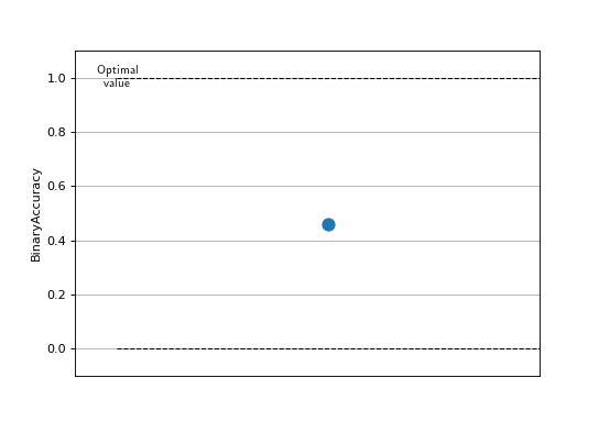
A single point plot is not that informative in itself, but if available we will try to include additional information
such as the lower and upper bounds the particular metric can take and if the metric should be minimized or maximized
to be optimal. This is true for all metrics that return a scalar tensor.
Some metrics return multiple values (such as an tensor with multiple elements or a dict of scalar tensors), and in
that case calling .plot will return a figure similar to this:
metric = torchmetrics.Accuracy(task="multiclass", num_classes=3, average=None)
for _ in range(num_updates):
    metric.update(torch.randint(3, (10,)), torch.randint(3, (10,)))
fig, ax = metric.plot()
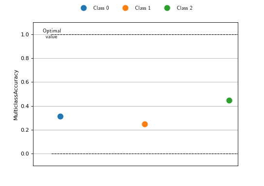
Here, each element is assumed to be an independent metric and plotted as its own point for comparing. The above is true
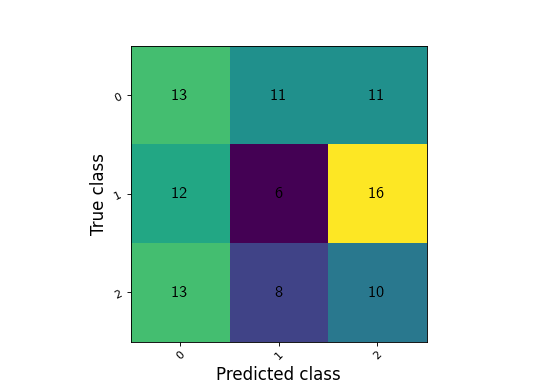
for all metrics that return a scalar tensor, but if the metric returns a tensor with multiple elements then the
.plot method will return a specialized plot for that particular metric. Take for example the ConfusionMatrix
metric:
metric = torchmetrics.ConfusionMatrix(task="multiclass", num_classes=3)
for _ in range(num_updates):
    metric.update(torch.randint(3, (10,)), torch.randint(3, (10,)))
fig, ax = metric.plot()
If you prefer to use the functional interface of Torchmetrics, you can also plot the values returned by the functional. However, you would still need to initialize the corresponding metric class to get the information about the metric:
plot_class = torchmetrics.Accuracy(task="multiclass", num_classes=3)
value = torchmetrics.functional.accuracy(
    torch.randint(3, (10,)), torch.randint(3, (10,)), num_classes=3
)
fig, ax = plot_class.plot(value)
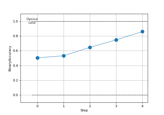
Plotting multi steps
In the above examples we have only plotted a single step/single value, but it is also possible to plot multiple steps
from the same metric. This is often the case when training a machine learning model, where you are tracking one or
multiple metrics that you want to plot as they are changing over time. This can be done by providing a sequence of outputs from
any metric, computed using metric.forward or metric.compute. For example, if we want to plot the accuracy of
a model over time, we could do it like this:
metric = torchmetrics.Accuracy(task="binary")
values = [ ]
for step in range(num_steps):
    for _ in range(num_updates):
        metric.update(preds(step), target(step))
    values.append(metric.compute())  # save value
    metric.reset()
fig, ax = metric.plot(values)
Do note that metrics that do not return simple scalar tensors, such as ConfusionMatrix, ROC that have specialized visualization does not support plotting multiple steps, out of the box and the user needs to manually plot the values for each step.
Plotting a collection of metrics
MetricCollection also supports .plot method and by default it works by just returning a collection of plots for
all its members. Thus, instead of returning a single (fig, ax) pair, calling .plot method of MetricCollection will
return a sequence of such pairs, one for each member in the collection. In the following example we are forming a
collection of binary classification metrics and redirecting the output of .plot to different subplots:
collection = torchmetrics.MetricCollection(
    torchmetrics.Accuracy(task="binary"),
    torchmetrics.Recall(task="binary"),
    torchmetrics.Precision(task="binary"),
)
fig, ax = plt.subplots(nrows=1, ncols=3)
values = [ ]
for step in range(num_steps):
    for _ in range(num_updates):
        collection.update(preds(step), target(step))
    values.append(collection.compute())
    collection.reset()
collection.plot(val=values, ax=ax)
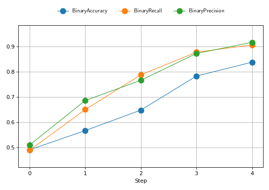
However, the plot method of MetricCollection also supports an additional argument called together that will
automatically try to plot all the metrics in the collection together in the same plot (with appropriate labels). This
is only possible if all the metrics in the collection return a scalar tensor.
collection = torchmetrics.MetricCollection(
    torchmetrics.Accuracy(task="binary"),
    torchmetrics.Recall(task="binary"),
    torchmetrics.Precision(task="binary"),
)
values = [ ]
fig, ax = plt.subplots(figsize=(6.8, 4.8))
for step in range(num_steps):
    for _ in range(num_updates):
        collection.update(preds(step), target(step))
    values.append(collection.compute())
    collection.reset()
collection.plot(val=values, together=True)
Advance example
In the following we are going to show how to use the .plot method to create a more advanced plot. We are going to
combine the functionality of several metrics using MetricCollection and plot them together. In addition we are going
to rely on MetricTracker to keep track of the metrics over multiple steps.
# Define collection that is a mix of metrics that return a scalar tensors and not
confmat = torchmetrics.ConfusionMatrix(task="binary")
roc = torchmetrics.ROC(task="binary")
collection = torchmetrics.MetricCollection(
    torchmetrics.Accuracy(task="binary"),
    torchmetrics.Recall(task="binary"),
    torchmetrics.Precision(task="binary"),
    confmat,
    roc,
)

# Define tracker over the collection to easy keep track of the metrics over multiple steps
tracker = torchmetrics.wrappers.MetricTracker(collection)

# Run "training" loop
for step in range(num_steps):
    tracker.increment()
    for _ in range(N):
        tracker.update(preds(step), target(step))

# Extract all metrics from all steps
all_results = tracker.compute_all()

# Construct a single figure with appropriate layout for all metrics
fig = plt.figure(layout="constrained")
ax1 = plt.subplot(2, 2, 1)
ax2 = plt.subplot(2, 2, 2)
ax3 = plt.subplot(2, 2, (3, 4))

# ConfusionMatrix and ROC we just plot the last step, notice how we call the plot method of those metrics
confmat.plot(val=all_results[-1]['BinaryConfusionMatrix'], ax=ax1)
roc.plot(all_results[-1]["BinaryROC"], ax=ax2)

# For the remaining we plot the full history, but we need to extract the scalar values from the results
scalar_results = [
    {k: v for k, v in ar.items() if isinstance(v, torch.Tensor) and v.numel() == 1} for ar in all_results
]
tracker.plot(val=scalar_results, ax=ax3)
